Front visualization

The jmetal.lab.visualization submodule contains several classes useful for plotting solutions. jMetalPy includes three types of visualization charts: static, interactive and streaming.

Static plots

It is possible to visualize the final front approximation by using the Plot class:

from jmetal.lab.visualization import Plot

plot_front = Plot(title='Pareto front approximation', axis_labels=['x', 'y'])
plot_front.plot(front, label='NSGAII-ZDT1')

Note

Static charts can be shown on the screen or stored in a file by setting the filename.

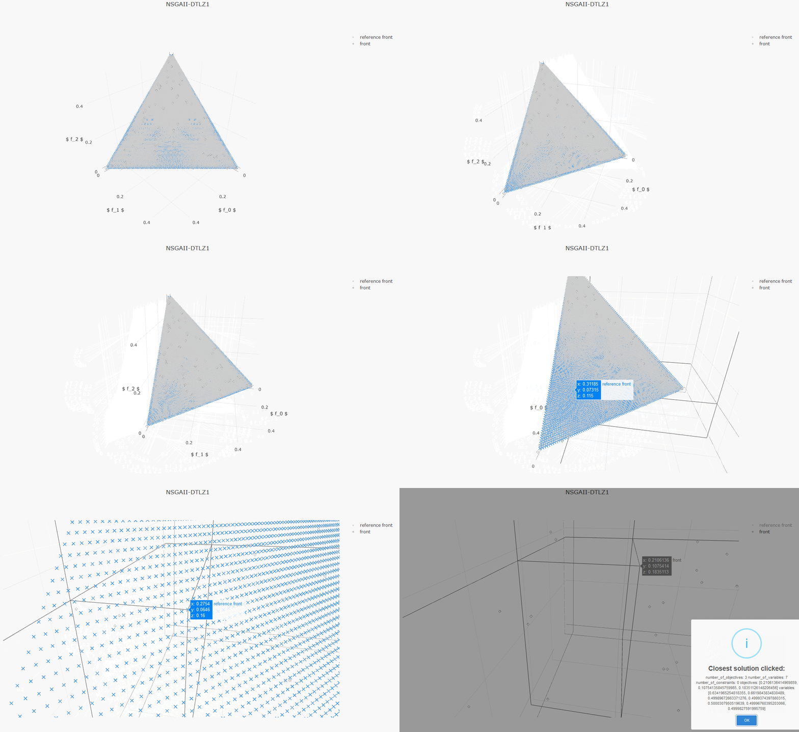
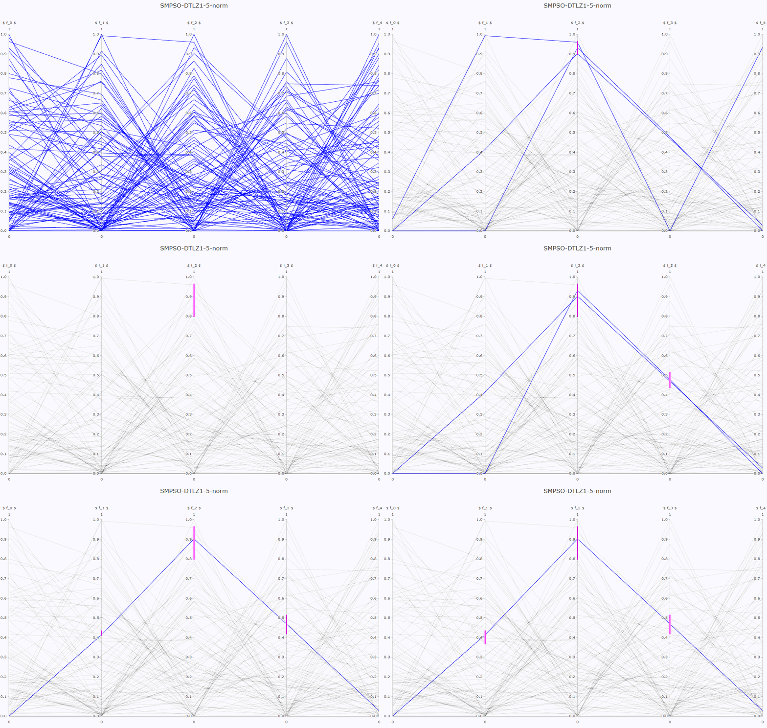
For problems with two and three objectives, the figure produced is a scatter plot; for problems with more than three objectives, a parallel coordinates plot is used. Note that any arbitrary number of fronts can be plotted for comparison purposes:

plot_front = Plot(title='Pareto front approximation', axis_labels=['x', 'y'])
plot_front.plot([front1, front2], label=['zdt1', 'zdt2'], filename='output', format='eps')

API

plotting

Plot(title='Pareto front approximation', reference_front=None, reference_point=None, axis_labels=None)

:param title: Title of the graph. :param axis_labels: List of axis labels. :param reference_point: Reference point (e.g., [0.4, 1.2]). :param reference_front: Reference Pareto front (if any) as solutions.

Source code in src/jmetal/lab/visualization/plotting.py

def __init__(
    self,
    title: str = "Pareto front approximation",
    reference_front: list[S] = None,
    reference_point: list = None,
    axis_labels: list = None,
):
    """
    :param title: Title of the graph.
    :param axis_labels: List of axis labels.
    :param reference_point: Reference point (e.g., [0.4, 1.2]).
    :param reference_front: Reference Pareto front (if any) as solutions.
    """
    self.plot_title = title
    self.axis_labels = axis_labels

    if reference_point and not isinstance(reference_point[0], list):
        reference_point = [reference_point]

    self.reference_point = reference_point
    self.reference_front = reference_front
    self.dimension = None

get_points(solutions) staticmethod

Get points for each solution of the front.

:param solutions: List of solutions. :return: Pandas dataframe with one column for each objective and one row for each solution.

Source code in src/jmetal/lab/visualization/plotting.py

@staticmethod
def get_points(solutions: list[S]) -> tuple[pd.DataFrame, int]:
    """Get points for each solution of the front.

    :param solutions: List of solutions.
    :return: Pandas dataframe with one column for each objective and one row for each solution.
    """
    if solutions is None:
        raise Exception("Front is none!")

    points = pd.DataFrame(list(solution.objectives for solution in solutions))
    return points, points.shape[1]

plot(front, label='', normalize=False, filename=None, format='eps')

Plot any arbitrary number of fronts in 2D, 3D or p-coords.

:param front: Pareto front or a list of them. :param label: Pareto front title or a list of them. :param normalize: If True, normalize data (for p-coords). :param filename: Output filename. :param format: Output file format.

Source code in src/jmetal/lab/visualization/plotting.py

def plot(
    self, front, label="", normalize: bool = False, filename: str = None, format: str = "eps"
):
    """Plot any arbitrary number of fronts in 2D, 3D or p-coords.

    :param front: Pareto front or a list of them.
    :param label: Pareto front title or a list of them.
    :param normalize: If True, normalize data (for p-coords).
    :param filename: Output filename.
    :param format: Output file format.
    """
    if not isinstance(front[0], list):
        front = [front]

    if not isinstance(label, list):
        label = [label]

    if len(front) != len(label):
        raise Exception("Number of fronts and labels must be the same")

    dimension = len(front[0][0].objectives)

    if dimension == 2:
        self.two_dim(front, label, filename, format)
    elif dimension == 3:
        self.three_dim(front, label, filename, format)
    else:
        self.pcoords(front, normalize, filename, format)

two_dim(fronts, labels=None, filename=None, format='eps')

Plot any arbitrary number of fronts in 2D.

:param fronts: List of fronts (containing solutions). :param labels: List of fronts title (if any). :param filename: Output filename.

Source code in src/jmetal/lab/visualization/plotting.py

def two_dim(
    self,
    fronts: list[list],
    labels: list[str] = None,
    filename: str = None,
    format: str = "eps",
):
    """Plot any arbitrary number of fronts in 2D.

    :param fronts: List of fronts (containing solutions).
    :param labels: List of fronts title (if any).
    :param filename: Output filename.
    """
    n = int(np.ceil(np.sqrt(len(fronts))))
    fig = plt.figure()
    fig.suptitle(self.plot_title, fontsize=16)

    reference = None
    if self.reference_front:
        reference, _ = self.get_points(self.reference_front)

    for i, _ in enumerate(fronts):
        points, _ = self.get_points(fronts[i])

        ax = fig.add_subplot(n, n, i + 1)
        points.plot(kind="scatter", x=0, y=1, ax=ax, s=10, color="#236FA4", alpha=1.0)

        if labels:
            ax.set_title(labels[i])

        if self.reference_front:
            reference.plot(x=0, y=1, ax=ax, color="k", legend=False)

        if self.reference_point:
            for point in self.reference_point:
                plt.plot([point[0]], [point[1]], marker="o", markersize=5, color="r")
                plt.axvline(x=point[0], color="r", linestyle=":")
                plt.axhline(y=point[1], color="r", linestyle=":")

        if self.axis_labels:
            plt.xlabel(self.axis_labels[0])
            plt.ylabel(self.axis_labels[1])

    if filename:
        _filename = filename + "." + format

        plt.savefig(_filename, format=format, dpi=1000)
        logger.info("Figure {_filename} saved to file")
    else:
        plt.show()

    plt.close(fig=fig)

three_dim(fronts, labels=None, filename=None, format='eps')

Plot any arbitrary number of fronts in 3D.

:param fronts: List of fronts (containing solutions). :param labels: List of fronts title (if any). :param filename: Output filename.

Source code in src/jmetal/lab/visualization/plotting.py

def three_dim(
    self,
    fronts: list[list],
    labels: list[str] = None,
    filename: str = None,
    format: str = "eps",
):
    """Plot any arbitrary number of fronts in 3D.

    :param fronts: List of fronts (containing solutions).
    :param labels: List of fronts title (if any).
    :param filename: Output filename.
    """
    n = int(np.ceil(np.sqrt(len(fronts))))
    fig = plt.figure()
    fig.suptitle(self.plot_title, fontsize=16)

    for i, _ in enumerate(fronts):
        ax = fig.add_subplot(n, n, i + 1, projection="3d")

        # Drawn first (background) and styled to recede: reference fronts are
        # often a dense sampling of the whole true surface (e.g. 10000 points
        # for DTLZ1/DTLZ2's bundled .pf files) -- with matplotlib's defaults
        # for both scatters, that dense, opaquely-colored cloud drawn on top
        # of the sparser obtained front (e.g. 100 points) hid it completely.
        if self.reference_front:
            ax.scatter(
                [s.objectives[0] for s in self.reference_front],
                [s.objectives[1] for s in self.reference_front],
                [s.objectives[2] for s in self.reference_front],
                s=2,
                color="lightgray",
                alpha=0.3,
            )

        # Drawn last (foreground) so it stays visible over the reference front.
        ax.scatter(
            [s.objectives[0] for s in fronts[i]],
            [s.objectives[1] for s in fronts[i]],
            [s.objectives[2] for s in fronts[i]],
            s=15,
            color="#236FA4",
            alpha=1.0,
        )

        if labels:
            ax.set_title(labels[i])

        if self.reference_point:
            # todo
            pass

        ax.relim()
        ax.autoscale_view(True, True, True)
        ax.view_init(elev=30.0, azim=15.0)
        ax.locator_params(nbins=4)

    if filename:
        _filename = filename + "." + format

        plt.savefig(_filename, format=format, dpi=1000)
        logger.info("Figure {_filename} saved to file")
    else:
        plt.show()

    plt.close(fig=fig)

pcoords(fronts, normalize=False, filename=None, format='eps')

Plot any arbitrary number of fronts in parallel coordinates.

:param fronts: List of fronts (containing solutions). :param filename: Output filename.

Source code in src/jmetal/lab/visualization/plotting.py

def pcoords(
    self, fronts: list[list], normalize: bool = False, filename: str = None, format: str = "eps"
):
    """Plot any arbitrary number of fronts in parallel coordinates.

    :param fronts: List of fronts (containing solutions).
    :param filename: Output filename.
    """
    n = int(np.ceil(np.sqrt(len(fronts))))
    fig = plt.figure()
    fig.suptitle(self.plot_title, fontsize=16)

    for i, _ in enumerate(fronts):
        points, _ = self.get_points(fronts[i])

        if normalize:
            points = (points - points.min()) / (points.max() - points.min())

        ax = fig.add_subplot(n, n, i + 1)

        min_, max_ = points.values.min(), points.values.max()
        points["scale"] = np.linspace(0, 1, len(points)) * (max_ - min_) + min_
        pd.plotting.parallel_coordinates(points, "scale", ax=ax)

        ax.get_legend().remove()

        if self.axis_labels:
            ax.set_xticklabels(self.axis_labels)

    if filename:
        plt.savefig(filename + "." + format, format=format, dpi=1000)
    else:
        plt.show()

    plt.close(fig=fig)

Interactive plots

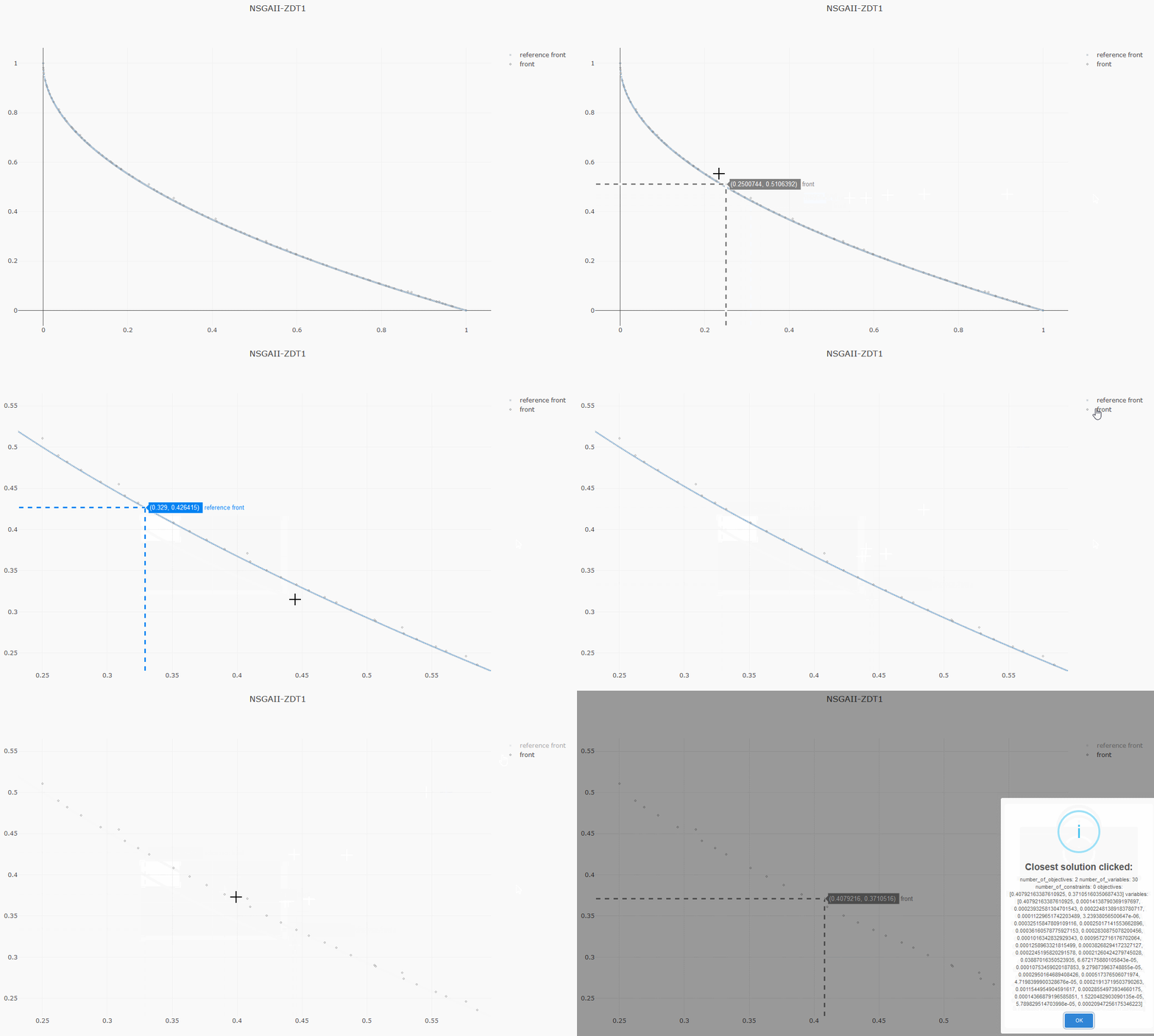
This kind of plot is interactive, in the sense that every solution can be manipulated (e.g., actions such as zoom, selecting part of the graph, or clicking on a point to see its objective values are allowed).

plot_front = InteractivePlot(title='Pareto front approximation')
plot_front.plot(front, label='NSGAII-ZDT1', filename='NSGAII-ZDT1-interactive')

API

interactive

InteractivePlot(title='Pareto front approximation', reference_front=None, reference_point=None, axis_labels=None)

Bases: Plot

Source code in src/jmetal/lab/visualization/interactive.py

def __init__(
    self,
    title: str = "Pareto front approximation",
    reference_front: list[S] = None,
    reference_point: list = None,
    axis_labels: list = None,
):
    super().__init__(title, reference_front, reference_point, axis_labels)
    self.figure = None
    self.layout = None
    self.data: list[Any] = []

plot(front, label=None, normalize=False, filename=None, format='HTML')

Plot a front of solutions (2D, 3D or parallel coordinates).

:param front: List of solutions. :param label: Front name. :param normalize: Normalize the input front between 0 and 1 (for problems with more than 3 objectives). :param filename: Output filename.

Source code in src/jmetal/lab/visualization/interactive.py

def plot(
    self, front, label=None, normalize: bool = False, filename: str = None, format: str = "HTML"
):
    """Plot a front of solutions (2D, 3D or parallel coordinates).

    :param front: List of solutions.
    :param label: Front name.
    :param normalize: Normalize the input front between 0 and 1 (for problems with more than 3 objectives).
    :param filename: Output filename.
    """
    if not isinstance(label, list):
        label = [label]

    self.layout = go.Layout(
        margin=dict(l=80, r=80, b=80, t=150),
        height=800,
        title=f"{self.plot_title}<br>{label[0]}",
        scene=dict(
            xaxis=dict(title=self.axis_labels[0:1][0] if self.axis_labels[0:1] else None),
            yaxis=dict(title=self.axis_labels[1:2][0] if self.axis_labels[1:2] else None),
            zaxis=dict(title=self.axis_labels[2:3][0] if self.axis_labels[2:3] else None),
        ),
        hovermode="closest",
    )

    # If any reference front, plot
    if self.reference_front:
        points, _ = self.get_points(self.reference_front)
        trace = self.__generate_trace(
            points=points, legend="Reference front", normalize=normalize, color="black", size=2
        )
        self.data.append(trace)

    # If any reference point, plot
    if self.reference_point:
        points = pd.DataFrame(self.reference_point)
        trace = self.__generate_trace(
            points=points, legend="Reference point", color="red", size=8
        )
        self.data.append(trace)

    # Get points and metadata
    points, _ = self.get_points(front)
    metadata = list(solution.__str__() for solution in front)

    trace = self.__generate_trace(
        points=points, metadata=metadata, legend="Front approximation", normalize=normalize
    )
    self.data.append(trace)
    self.figure = go.Figure(data=self.data, layout=self.layout)

    # Plot the figure
    if filename:
        if format == "HTML":
            self.export_to_html(filename)
            logger.info("Figure {_filename} exported to HTML file")
        else:
            _filename = filename + "." + format

            pio.write_image(self.figure, _filename)
            logger.info("Figure {_filename} saved to file")

export_to_html(filename)

Export the graph to an interactive HTML (solutions can be selected to show some metadata).

:param filename: Output file name. :return: Script as string.

Source code in src/jmetal/lab/visualization/interactive.py

def export_to_html(self, filename: str) -> str:
    """Export the graph to an interactive HTML (solutions can be selected to show some metadata).

    :param filename: Output file name.
    :return: Script as string."""
    html_string = (
        """
    <!DOCTYPE html>
    <html>
        <head>
            <meta charset="utf-8"/>
            <script src="https://cdn.plot.ly/plotly-latest.min.js"></script>
            <script src="https://unpkg.com/sweetalert2@7.7.0/dist/sweetalert2.all.js"></script>
            <link rel="stylesheet" href="https://maxcdn.bootstrapcdn.com/bootstrap/3.3.1/css/bootstrap.min.css">
        </head>
        <body>
            """
        + self.export_to_div(filename=None, include_plotlyjs=False)
        + """
            <script>
                var myPlot = document.querySelectorAll('div')[0];
                myPlot.on('plotly_click', function(data){
                    var pts = '';

                    for(var i=0; i < data.points.length; i++){
                        pts = '(x, y) = ('+data.points[i].x +', '+ data.points[i].y.toPrecision(4)+')';
                        cs = data.points[i].customdata
                    }

                    if(typeof cs !== "undefined"){
                        swal({
                          title: 'Closest solution clicked:',
                          text: cs,
                          type: 'info',
                          position: 'bottom-end'
                        })
                    }
                });

                window.onresize = function() {
                   Plotly.Plots.resize(myPlot);
                };
            </script>
        </body>
    </html>"""
    )

    with open(filename + ".html", "w") as outf:
        outf.write(html_string)

    return html_string

export_to_div(filename=None, include_plotlyjs=False)

Export as a div for embedding the graph in an HTML file.

:param filename: Output file name (if desired, default to None). :param include_plotlyjs: If True, include plot.ly JS script (default to False). :return: Script as string.

Source code in src/jmetal/lab/visualization/interactive.py

def export_to_div(self, filename=None, include_plotlyjs: bool = False) -> str:
    """Export as a `div` for embedding the graph in an HTML file.

    :param filename: Output file name (if desired, default to None).
    :param include_plotlyjs: If True, include plot.ly JS script (default to False).
    :return: Script as string.
    """
    script = offline.plot(
        self.figure, output_type="div", include_plotlyjs=include_plotlyjs, show_link=False
    )

    if filename:
        with open(filename + ".html", "w") as outf:
            outf.write(script)

    return script

Streaming plots

The visualizer observer displays the front in real-time (note it only works for problems with two and three objectives) during the execution of multi-objective algorithms; this can be useful to observe the evolution of the Pareto front approximation:

from jmetal.util.observer import VisualizerObserver

algorithm.observable.register(observer=VisualizerObserver(reference_front=problem.reference_front))

API

streaming

StreamingPlot(plot_title='Pareto front approximation', reference_front=None, reference_point=None, axis_labels=None)

:param plot_title: Title of the graph. :param axis_labels: List of axis labels. :param reference_point: Reference point (e.g., [0.4, 1.2]). :param reference_front: Reference Pareto front (if any) as solutions.

Source code in src/jmetal/lab/visualization/streaming.py

def __init__(
    self,
    plot_title: str = "Pareto front approximation",
    reference_front: list[S] = None,
    reference_point: list = None,
    axis_labels: list = None,
):
    """
    :param plot_title: Title of the graph.
    :param axis_labels: List of axis labels.
    :param reference_point: Reference point (e.g., [0.4, 1.2]).
    :param reference_front: Reference Pareto front (if any) as solutions.
    """
    self.plot_title = plot_title
    self.axis_labels = axis_labels

    if reference_point and not isinstance(reference_point[0], list):
        reference_point = [reference_point]

    self.reference_point = reference_point
    self.reference_front = reference_front
    self.dimension = None

    import warnings

    warnings.filterwarnings("ignore", ".*GUI is implemented.*")

    self.fig, self.ax = plt.subplots()
    self.sc = None
    self.axis = None

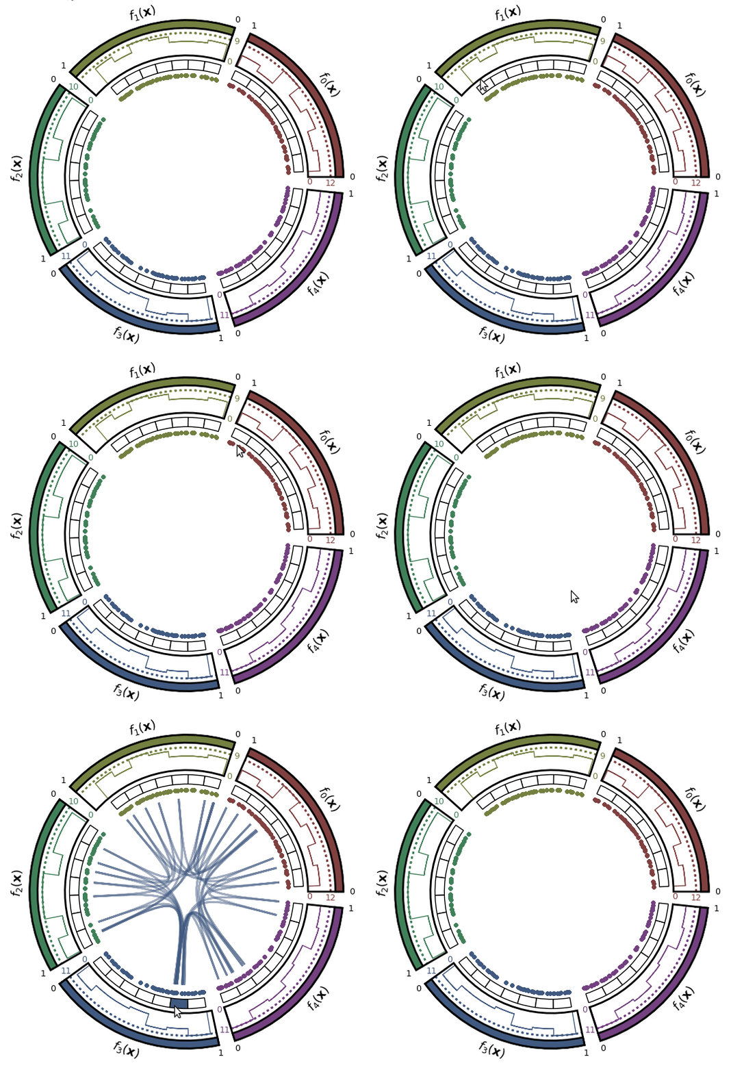
Chord plot

API

chord_plot

Posterior plot

API

posterior

plot_posterior(sample, higher_is_better=False, min_points_per_hexbin=2, alg_names=None, filename='posterior.eps')

Plots the sample from posterior distribution of a Bayesian statistical test.

Parameters:

Name	Type	Description	Default
sample	DataFrame | ndarray	An (n x 3) array or DataFrame containing the probabilities.	required
alg_names	list	Names of the algorithms under evaluation. Defaults to ['Alg1', 'Alg2'].	None

Returns:

Type	Description
Figure	The matplotlib Figure.

Source code in src/jmetal/lab/visualization/posterior.py

def plot_posterior(
    sample: pd.DataFrame | np.ndarray,
    higher_is_better: bool = False,
    min_points_per_hexbin: int = 2,
    alg_names: list = None,
    filename: str = "posterior.eps",
) -> plt.Figure:
    """Plots the sample from posterior distribution of a Bayesian statistical test.

    Args:
        sample: An (n x 3) array or DataFrame containing the probabilities.
        alg_names: Names of the algorithms under evaluation. Defaults to ``['Alg1', 'Alg2']``.

    Returns:
        The matplotlib Figure.
    """

    # Initial Checking
    if type(sample) == pd.DataFrame:
        sample = sample.values

    if sample.ndim == 2:
        nrow, ncol = sample.shape
        if ncol != 3:
            raise ValueError("Initialization ERROR. Incorrect number of dimensions in axis 1.")
    else:
        raise ValueError("Initialization ERROR. Incorrect number of dimensions for sample")

    def transform(p):
        lambda1, lambda2, lambda3 = p.T
        x = 0.1 * lambda1 + 0.5 * lambda2 + 0.9 * lambda3
        y = (0.2 * lambda1 + 1.4 * lambda2 + 0.2 * lambda3) / np.sqrt(3)
        return np.vstack((x, y)).T

    # Initialize figure
    fig = plt.figure(figsize=(5, 5), facecolor="white")
    ax = fig.add_axes([0, 0, 1, 1])
    ax.set_xlim(0, 1)
    ax.set_ylim(0, 1)
    ax.set_axis_off()

    # plot text

    if not higher_is_better:
        if not alg_names:
            ax.text(x=0.5, y=1.4 / np.sqrt(3) + 0.005, s="P(rope)", ha="center", va="bottom")
            ax.text(x=0.15, y=0.175 / np.sqrt(3) - 0.005, s="P(alg1<alg2)", ha="right", va="top")
            ax.text(x=0.85, y=0.175 / np.sqrt(3) - 0.005, s="P(alg1>alg2)", ha="left", va="top")
        else:
            ax.text(x=0.5, y=1.4 / np.sqrt(3) + 0.005, s="P(rope)", ha="center", va="bottom")
            ax.text(
                x=0.15,
                y=0.175 / np.sqrt(3) - 0.005,
                s="P(" + alg_names[0] + ")",
                ha="right",
                va="top",
            )
            ax.text(
                x=0.85,
                y=0.175 / np.sqrt(3) - 0.005,
                s="P(" + alg_names[1] + ")",
                ha="left",
                va="top",
            )
    else:
        if not alg_names:
            ax.text(x=0.5, y=1.4 / np.sqrt(3) + 0.005, s="P(rope)", ha="center", va="bottom")
            ax.text(x=0.15, y=0.175 / np.sqrt(3) - 0.005, s="P(alg2<alg1)", ha="right", va="top")
            ax.text(x=0.85, y=0.175 / np.sqrt(3) - 0.005, s="P(alg2>alg1)", ha="left", va="top")
        else:
            ax.text(x=0.5, y=1.4 / np.sqrt(3) + 0.005, s="P(rope)", ha="center", va="bottom")
            ax.text(
                x=0.15,
                y=0.175 / np.sqrt(3) - 0.005,
                s="P(" + alg_names[1] + ")",
                ha="right",
                va="top",
            )
            ax.text(
                x=0.85,
                y=0.175 / np.sqrt(3) - 0.005,
                s="P(" + alg_names[0] + ")",
                ha="left",
                va="top",
            )

    # Conversion between barycentric and Cartesian coordinates
    sample2d = np.zeros((sample.shape[0], 2))
    for p in range(sample.shape[0]):
        sample2d[p, :] = transform(sample[p, :])

    # Plot projected points
    ax.hexbin(sample2d[:, 0], sample2d[:, 1], mincnt=min_points_per_hexbin, cmap=plt.cm.plasma)

    # Plot triangle

    ax.plot([0.095, 0.505], [0.2 / np.sqrt(3), 1.4 / np.sqrt(3)], linewidth=3.0, color="white")
    ax.plot([0.505, 0.905], [1.4 / np.sqrt(3), 0.2 / np.sqrt(3)], linewidth=3.0, color="white")
    ax.plot([0.09, 0.905], [0.2 / np.sqrt(3), 0.2 / np.sqrt(3)], linewidth=3.0, color="white")

    ax.plot([0.1, 0.5], [0.2 / np.sqrt(3), 1.4 / np.sqrt(3)], linewidth=3.0, color="gray")
    ax.plot([0.5, 0.9], [1.4 / np.sqrt(3), 0.2 / np.sqrt(3)], linewidth=3.0, color="gray")
    ax.plot([0.1, 0.9], [0.2 / np.sqrt(3), 0.2 / np.sqrt(3)], linewidth=3.0, color="gray")

    # plot division lines
    ax.plot([0.5, 0.5], [0.2 / np.sqrt(3), 0.6 / np.sqrt(3)], linewidth=3.0, color="gray")
    ax.plot([0.3, 0.5], [0.8 / np.sqrt(3), 0.6 / np.sqrt(3)], linewidth=3.0, color="gray")
    ax.plot([0.5, 0.7], [0.6 / np.sqrt(3), 0.8 / np.sqrt(3)], linewidth=3.0, color="gray")

    if filename:
        plt.savefig(filename, bbox_inches="tight")
        logger.info(f"Figure {filename} saved to file")

    plt.show()